The action depends on the type of the object, and
this is set up by the function that created the object;
see “Details”. These are basic plot styles, with
somewhat limited scope for customization. Since the data with
argoFloats objects are easy to extract, users should
not find it difficult to create their own plots to meet a
particular aesthetic. See “Examples” and Kelley et al. (2021)
for more plotting examples.
# S4 method for class 'argoFloats'
plot(
  x,
  which = "map",
  bathymetry = argoDefaultBathymetry(),
  geographical = 0,
  xlim = NULL,
  ylim = NULL,
  xlab = NULL,
  ylab = NULL,
  type = "p",
  cex = par("cex"),
  col = par("fg"),
  pch = par("pch"),
  bg = par("bg"),
  eos = "gsw",
  mapControl = NULL,
  profileControl = NULL,
  QCControl = NULL,
  summaryControl = NULL,
  TSControl = NULL,
  debug = 0,
  ...
)
Arguments
- x
an
argoFloatsobject.- which
a character value indicating the type of plot. The possible choices are
"map","profile","QC","summary"and"TS"; see “Details”.- bathymetry
an argument used only if
which="map", to control whether (and how) to indicate water depth. Note that the default wasTRUEuntil 2021-12-02, but was changed toFALSEon that date, to avoid a bathymetry download, which can be a slow operations. See “Details” for details, and Example 4 for a hint on compensating for the margin adjustment done if an image is used to show bathymetry.- geographical
flag indicating the style of axes for the
which="map"case, but only if no projection is called for in themapControlargument. Withgeographical=0(which is the default), the axis ticks are labeled with signed longitudes and latitudes, measured in degrees. The signs are dropped withgeographical=1. In thegeographical=4case, signs are also dropped, but hemispheres are indicated by writingS,N,WorEafter axis tick labels, except at the equator and prime meridian. Note that this scheme mimics that used byoce::plot,coastline-method().- xlim, ylim
numerical values, each a two-element vector, that set the
xandylimits of plot axes, as forplot.default()and other conventional plotting functions.- xlab
a character value indicating the name for the horizontal axis, or
NULL, which indicates that this function should choose an appropriate name depending on the value ofwhich. Note thatxlabis not obeyed ifwhich="TS", because altering that label can be confusing to the user.- ylab
as
xlab, but for the vertical axis.- type
a character value that controls the line type, with
"p"for unconnected points,"l"for line segments between undrawn points, etc.; see the docs forpar(), Iftypenot specified, it defaults to"p".- cex
a character expansion factor for plot symbols, or
NULL, to get an value that depends on the value ofwhich.- col
the colour to be used for plot symbols, or
NULL, to get an value that depends on the value ofwhich(see “Details”). Ifwhich="TS", then theTSControlargument takes precedence overcol.- pch
an integer or character value indicating the type of plot symbol, or
NULL, to get a value that depends on the value ofwhich. (Seepar()for more on specifyingpch.)- bg
the colour to be used for plot symbol interior, for
pchvalues that distinguish between the interior of the symbol and the border, e.g. forpch=21.- eos
a character value indicating the equation of state to use if
which="TS". This must be"gsw"(the default) or"unesco"; seeoce::plotTS().- mapControl
a list that permits particular control of the
which="map"case. If provided, it may contain elements namedbathymetry(which has the same effect as the parameterbathymetry),colLand(which indicates the colour of the land), andprojection(which may beFALSE, meaning to plot longitude and latitude on rectilinear axes,TRUE, meaning to plot withoce::mapPlot(), using Mollweide projection that is suitable mainly for world-scale views, or a character value that will be supplied tooce::mapPlot(). If a projection is used, then the positions of the Argo floats are plotted withoce::mapPoints(), rather than withpoints(), and if the user wishes to locate points with mouse clicks, thenoce::mapLocator()must be used instead oflocator(). Ifbathymetryis not contained inmapControl, it defaults toFALSE, and ifprojectionis not supplied, it defaults toFALSE. Note thatmapControltakes precedence over thebathymetryargument, if both are provided. Also note that, at present, bathymetry cannot be shown with map projections.- profileControl
a list that permits control of the
which="profile"case. If provided, it may contain elements namedparameter(a character value naming the quantity to plot on the x axis),ytype(a character value equal to either"pressure"or"sigma0") andconnect(a logical value indicating whether to skip acrossNAvalues if thetypeargument is"l","o", or"b"). IfprofileControlis not provided, it defaults tolist(parameter="temperature", ytype="pressure", connect=FALSE). Alternatively, ifprofileControlis missing any of the three elements, then they are given defaults as in the previous sentence.- QCControl
a list that permits control of the
which="QC"case. If provided, it may contain an element namedparameter, a character value naming the quantity for which the quality-control information is to be plotted, and an element nameddataStateIndicator, a logical value controlling whether to add a panel showing this quantity (see Reference Table 6 of reference 1 to learn more about what is encoded indataStateIndicator). If not provided,QCControldefaults tolist(parameter="temperature",dataStateIndicator=FALSE).- summaryControl
a list that permits control of the
which="summary". If provided, it should contain an element nameditems, a character vector naming the items to be shown. The possible entries in this vector are"dataStateIndicator"(see Reference Table 6 of reference 1, for more information on this quantity),"length"(the number of levels in the profile),"deepest"(the highest pressure recorded),"longitude"and"latitude". IfsummaryControlis not provided, all of these will be shown. If all the elements ofxhave the sameID, then the top panel will have ticks on its top axis, indicating thecycle.- TSControl
a list that permits control of the
which="TS"case, and is ignored for the other cases. IfTSControlis supplied, then other arguments that normally control plots are ignored.TSControlmay have elements nameddrawByCycle,cex,col,pch,lty,lwdandtype. The first of these is a logical value indicating whether to plot individual cycles with different aesthetic characteristics, and the other elements describe those characteristics in the usual way. By default,typeis"p", and the point characteristics are given by the other parameters, which are passed to [rep()] to have one value per cycle. For example,TSControl=list(drawByCycle=TRUE,col=1:2,type="l")` indicates to draw lines for the individual cycles, with the first being black, the second red, the third black, etc. FIXME: THIS IS NOT CODED YET.- debug
an integer specifying the level of debugging.
- ...
extra arguments passed to the plot calls that are made within this function.
Value
None (invisible NULL).
Details
The various plot types are as follows.
For
which="map", a map of profile locations is created if subtype is equal to cycles, or a rectangle highlighting the trajectory of a float ID is created when subtype is equal to trajectories. This only works if thetypeis"index"(meaning thatxwas created bygetIndex()or a subset of such an object, created withsubset,argoFloats-method()), orargos(meaning thatxwas created withreadProfiles(). The plot range is auto-selected. If theocedatapackage is available, then itscoastlineWorldFinedataset is used to draw a coastline (which will be visible only if the plot region is large enough); otherwise, if theocepackage is available, then itscoastlineWorlddataset is used. Thebathymetryargument controls whether (and how) to draw a map underlay that shows water depth. There are three possible values forbathymetry:FALSE(the default, viaargoDefaultBathymetry()), meaning not to draw bathymetry;TRUE, meaning to draw bathymetry as an image, using data downloaded withoce::download.topo(). Example 4 illustrates this, and also shows how to adjust the margins after the plot, in case there is a need to add extra graphical elements usingpoints(),lines(), etc.A list with items controlling both the bathymetry data and its representation in the plot (see Example 4). Those items are:
source, a mandatory value that is either (a) the string"auto"(the default) to useoce::download.topo()to download the data or (b) a value returned byoce::read.topo().contour, an optional logical value (withFALSEas the default) indicating whether to represent bathymetry with contours (with depths of 100m, 200m, 500m shown, along with 1km, 2km up to 10km), as opposed to an image;colormap, ignored ifcontourisTRUE, an optional value that is either the string"auto"(the default) for a form of GEBCO colors computed withoce::oceColorsGebco(), or a value computed withoce::colormap()applied to the bathymetry data; andpalette, ignored ifcontourisTRUE, an optional logical value (withTRUEas the default) indicating whether to draw a depth-color palette to the right of the plot. Note that the default value forbathymetryis set by a call toargoDefaultBathymetry(), and that this second function can only handle possibilities 1 and 2 above.
For
which="profile", a profile plot is created, showing the variation of some quantity with pressure or potential density anomaly, as specified by theprofileControlargument.For
which="QC", two time-series panels are shown, with time being that recorded in the individual profile in the dataset. An additional argument namedparametermust be given, to name the quantity of interest. The function only works ifxis anargoFloatsobject created withreadProfiles(). The top panel shows the percent of data flagged with codes 1 (meaning good data), 2 (probably good), 5 (changed) or 8 (estimated), as a function of time (lower axis) and (if all cycles are from a single Argo float) cycle number (upper axis, with smaller font). Thus, low values on the top panel reveal profiles that are questionable. Note that if all of data at a given time have flag 0, meaning not assessed, then a quality of 0 is plotted at that time. The bottom panel shows the mean value of the parameter in question regardless of the flag value.For
which="summary", one or more time-series panels are shown in a vertical stack. If there is only one ID inx, then the cycle values are indicated along the top axis of the top panel. The choice of panels is set by thesummaryControlargument.For
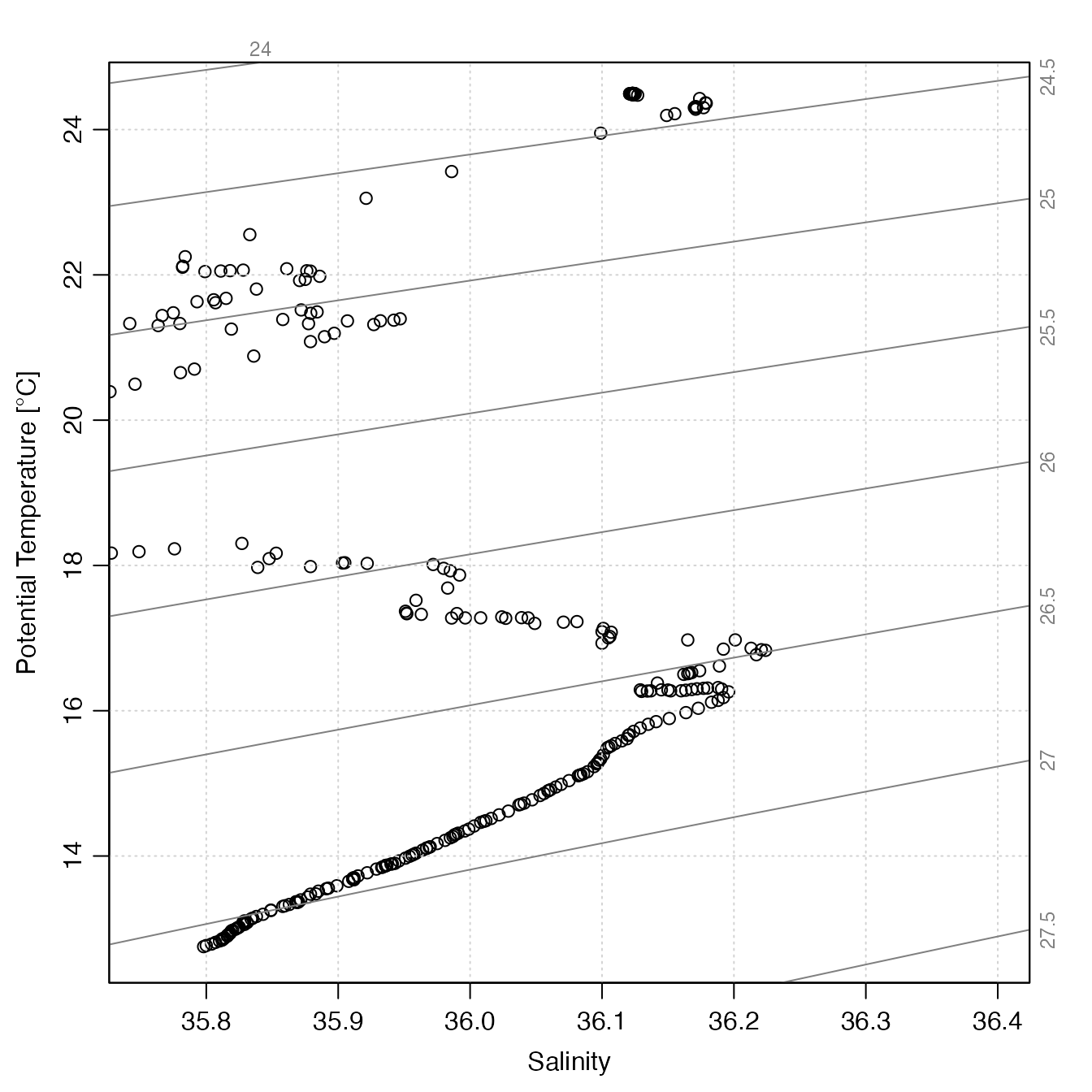
which="TS", a TS plot is created, by callingplotArgoTS()with the specifiedx,xlim,ylim,xlab,ylab,type,cex,col,pch,bg,eos, andTSControl, along withdebug-1. See the help forplotArgoTS()for how these parameters are interpreted.
References
Carval, Thierry, Bob Keeley, Yasushi Takatsuki, Takashi Yoshida, Stephen Loch, Claudia Schmid, and Roger Goldsmith. Argo User's Manual V3.3. Ifremer, 2019.
doi:10.13155/29825Kelley, D. E., Harbin, J., & Richards, C. (2021). argoFloats: An R package for analyzing Argo data. Frontiers in Marine Science, (8), 636922. doi:10.3389/fmars.2021.635922
Examples
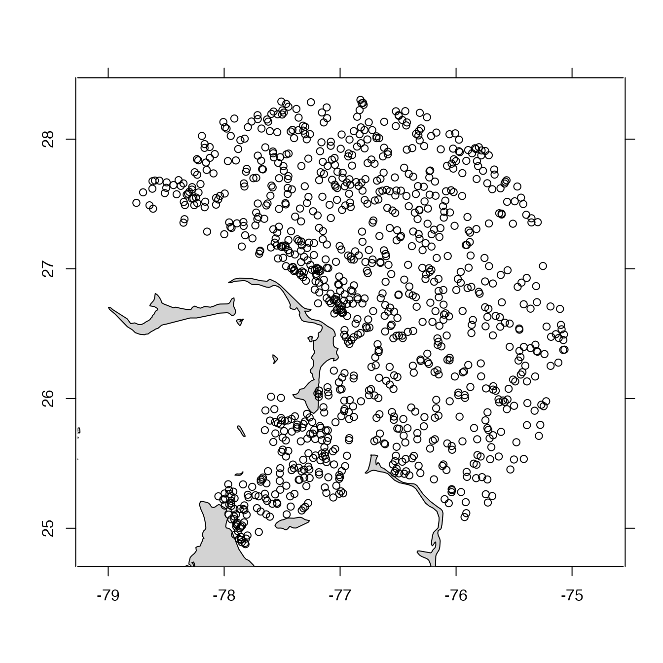
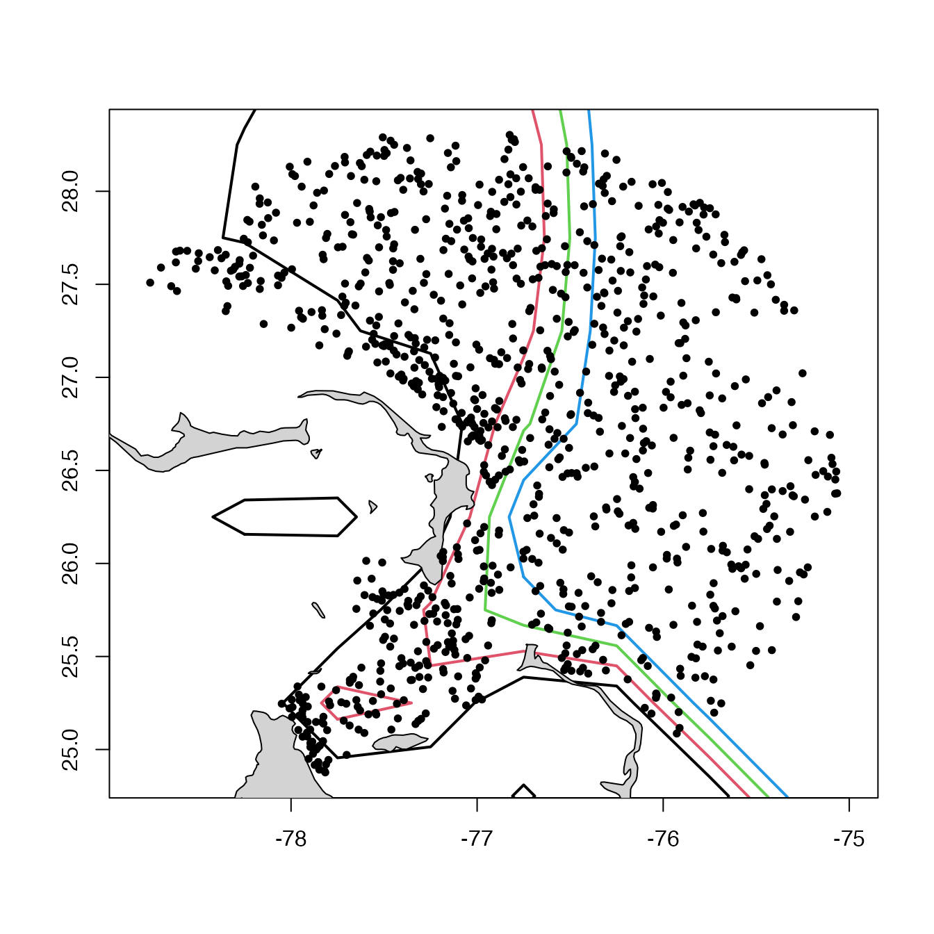
# Example 1: map profiles in index
library(argoFloats)
data(index)
plot(index)
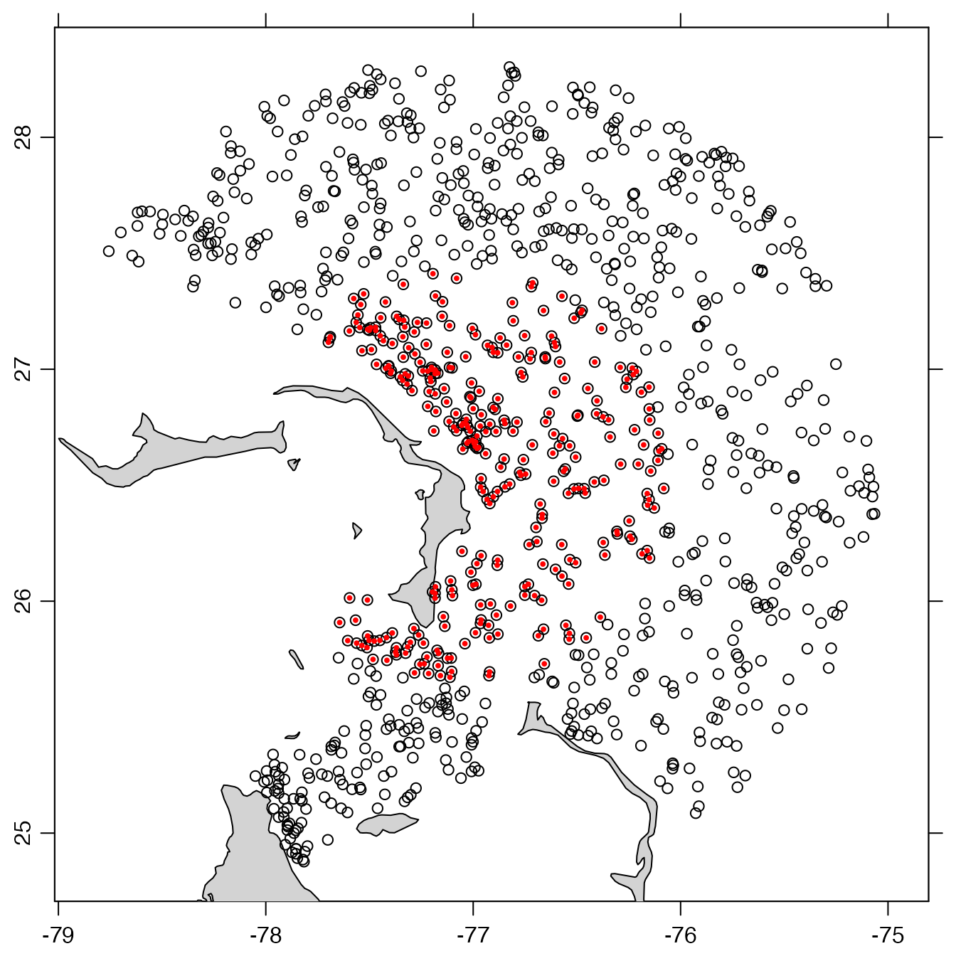
 # Example 2: as Example 1, but narrow the margins and highlight floats
# within a circular region of diameter 100 km.
oldpar <- par(no.readonly = TRUE)
par(mar = c(2, 2, 1, 1), mgp = c(2, 0.7, 0))
plot(index)
lon <- index[["longitude"]]
lat <- index[["latitude"]]
near <- oce::geodDist(lon, lat, -77.06, 26.54) < 100
R <- subset(index, near)
#> Kept 315 cycles (31.2%)
points(R[["longitude"]], R[["latitude"]],
cex = 0.6, pch = 20, col = "red"
)
# Example 2: as Example 1, but narrow the margins and highlight floats
# within a circular region of diameter 100 km.
oldpar <- par(no.readonly = TRUE)
par(mar = c(2, 2, 1, 1), mgp = c(2, 0.7, 0))
plot(index)
lon <- index[["longitude"]]
lat <- index[["latitude"]]
near <- oce::geodDist(lon, lat, -77.06, 26.54) < 100
R <- subset(index, near)
#> Kept 315 cycles (31.2%)
points(R[["longitude"]], R[["latitude"]],
cex = 0.6, pch = 20, col = "red"
)
 par(oldpar)
# Example 3: TS of a built-in data file.
f <- system.file("extdata", "SR2902204_131.nc", package = "argoFloats")
a <- readProfiles(f)
#> Warning: Of 1 profiles read, 1 has >10% of BBP700 values with QC flag of 4, signalling bad data.
#> The indices of the bad profiles are as follows.
#> 1
#> Warning: Of 1 profiles read, 1 has >10% of chlorophyllA values with QC flag of 4, signalling bad data.
#> The indices of the bad profiles are as follows.
#> 1
#> Warning: Of 1 profiles read, 1 has >10% of oxygen values with QC flag of 4, signalling bad data.
#> The indices of the bad profiles are as follows.
#> 1
#> Warning: Of 1 profiles read, 1 has >10% of pressure values with QC flag of 4, signalling bad data.
#> The indices of the bad profiles are as follows.
#> 1
oldpar <- par(no.readonly = TRUE)
par(mar = c(3.3, 3.3, 1, 1), mgp = c(2, 0.7, 0)) # wide margins for axis names
plot(a, which = "TS")
par(oldpar)
# Example 3: TS of a built-in data file.
f <- system.file("extdata", "SR2902204_131.nc", package = "argoFloats")
a <- readProfiles(f)
#> Warning: Of 1 profiles read, 1 has >10% of BBP700 values with QC flag of 4, signalling bad data.
#> The indices of the bad profiles are as follows.
#> 1
#> Warning: Of 1 profiles read, 1 has >10% of chlorophyllA values with QC flag of 4, signalling bad data.
#> The indices of the bad profiles are as follows.
#> 1
#> Warning: Of 1 profiles read, 1 has >10% of oxygen values with QC flag of 4, signalling bad data.
#> The indices of the bad profiles are as follows.
#> 1
#> Warning: Of 1 profiles read, 1 has >10% of pressure values with QC flag of 4, signalling bad data.
#> The indices of the bad profiles are as follows.
#> 1
oldpar <- par(no.readonly = TRUE)
par(mar = c(3.3, 3.3, 1, 1), mgp = c(2, 0.7, 0)) # wide margins for axis names
plot(a, which = "TS")
 #> NULL
par(oldpar)
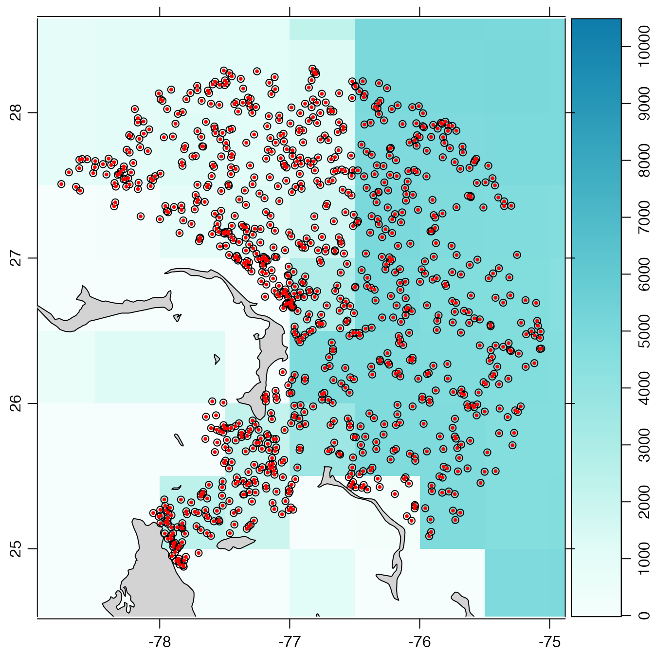
# \donttest{
# Example 4: map with bathymetry. Note that par(mar) is adjusted
# for the bathymetry palette, so it must be adjusted again after
# the plot(), in order to add new plot elements.
# This example specifies a coarse bathymetry dataset that is provided
# by the 'oce' package. In typical applications, the user will use
# a finer-scale dataset, either by using bathymetry=TRUE (which
# downloads a file appropriate for the plot view), or by using
# an already-downloaded file.
data(topoWorld, package = "oce")
oldpar <- par(no.readonly = TRUE)
par(mar = c(2, 2, 1, 2), mgp = c(2, 0.7, 0)) # narrow margins for a map
plot(index, bathymetry = list(source = topoWorld))
# For bathymetry plots that use images, plot() temporarily
# adds 2.75 to par("mar")[4] so the same must be done, in order
# to correctly position additional points (shown as black rings).
par(mar = par("mar") + c(0, 0, 0, 2.75))
points(index[["longitude"]], index[["latitude"]],
cex = 0.6, pch = 20, col = "red"
)
#> NULL
par(oldpar)
# \donttest{
# Example 4: map with bathymetry. Note that par(mar) is adjusted
# for the bathymetry palette, so it must be adjusted again after
# the plot(), in order to add new plot elements.
# This example specifies a coarse bathymetry dataset that is provided
# by the 'oce' package. In typical applications, the user will use
# a finer-scale dataset, either by using bathymetry=TRUE (which
# downloads a file appropriate for the plot view), or by using
# an already-downloaded file.
data(topoWorld, package = "oce")
oldpar <- par(no.readonly = TRUE)
par(mar = c(2, 2, 1, 2), mgp = c(2, 0.7, 0)) # narrow margins for a map
plot(index, bathymetry = list(source = topoWorld))
# For bathymetry plots that use images, plot() temporarily
# adds 2.75 to par("mar")[4] so the same must be done, in order
# to correctly position additional points (shown as black rings).
par(mar = par("mar") + c(0, 0, 0, 2.75))
points(index[["longitude"]], index[["latitude"]],
cex = 0.6, pch = 20, col = "red"
)
 par(oldpar)
# Example 5. Simple contour version, using coarse dataset (ok on basin-scale).
# Hint: use oce::download.topo() to download high-resolution datasets to
# use instead of topoWorld.
oldpar <- par(no.readonly = TRUE)
par(mar = c(2, 2, 1, 1))
data(topoWorld, package = "oce")
plot(index, bathymetry = list(source = topoWorld, contour = TRUE))
par(oldpar)
# Example 5. Simple contour version, using coarse dataset (ok on basin-scale).
# Hint: use oce::download.topo() to download high-resolution datasets to
# use instead of topoWorld.
oldpar <- par(no.readonly = TRUE)
par(mar = c(2, 2, 1, 1))
data(topoWorld, package = "oce")
plot(index, bathymetry = list(source = topoWorld, contour = TRUE))
 par(oldpar)
# Example 6. Customized map, sidestepping plot,argoFloats-method().
lon <- topoWorld[["longitude"]]
lat <- topoWorld[["latitude"]]
asp <- 1 / cos(pi / 180 * mean(lat))
# Limit plot region to float region.
xlim <- range(index[["longitude"]])
ylim <- range(index[["latitude"]])
# Colourize 1km, 2km, etc, isobaths.
contour(
x = lon, y = lat, z = topoWorld[["z"]], xlab = "", ylab = "",
xlim = xlim, ylim = ylim, asp = asp,
col = 1:6, lwd = 2, levels = -1000 * 1:6, drawlabels = FALSE
)
# Show land
data(coastlineWorldFine, package = "ocedata")
polygon(coastlineWorldFine[["longitude"]],
coastlineWorldFine[["latitude"]],
col = "lightgray"
)
# Indicate float positions.
points(index[["longitude"]], index[["latitude"]], pch = 20)
par(oldpar)
# Example 6. Customized map, sidestepping plot,argoFloats-method().
lon <- topoWorld[["longitude"]]
lat <- topoWorld[["latitude"]]
asp <- 1 / cos(pi / 180 * mean(lat))
# Limit plot region to float region.
xlim <- range(index[["longitude"]])
ylim <- range(index[["latitude"]])
# Colourize 1km, 2km, etc, isobaths.
contour(
x = lon, y = lat, z = topoWorld[["z"]], xlab = "", ylab = "",
xlim = xlim, ylim = ylim, asp = asp,
col = 1:6, lwd = 2, levels = -1000 * 1:6, drawlabels = FALSE
)
# Show land
data(coastlineWorldFine, package = "ocedata")
polygon(coastlineWorldFine[["longitude"]],
coastlineWorldFine[["latitude"]],
col = "lightgray"
)
# Indicate float positions.
points(index[["longitude"]], index[["latitude"]], pch = 20)
 # Example 7: Temperature profile of the 131st cycle of float with ID 2902204
a <- readProfiles(system.file("extdata", "SR2902204_131.nc", package = "argoFloats"))
#> Warning: Of 1 profiles read, 1 has >10% of BBP700 values with QC flag of 4, signalling bad data.
#> The indices of the bad profiles are as follows.
#> 1
#> Warning: Of 1 profiles read, 1 has >10% of chlorophyllA values with QC flag of 4, signalling bad data.
#> The indices of the bad profiles are as follows.
#> 1
#> Warning: Of 1 profiles read, 1 has >10% of oxygen values with QC flag of 4, signalling bad data.
#> The indices of the bad profiles are as follows.
#> 1
#> Warning: Of 1 profiles read, 1 has >10% of pressure values with QC flag of 4, signalling bad data.
#> The indices of the bad profiles are as follows.
#> 1
oldpar <- par(no.readonly = TRUE)
par(mfrow = c(1, 1))
par(mgp = c(2, 0.7, 0)) # mimic the oce::plotProfile() default
par(mar = c(1, 3.5, 3.5, 2)) # mimic the oce::plotProfile() default
plot(a, which = "profile")
# Example 7: Temperature profile of the 131st cycle of float with ID 2902204
a <- readProfiles(system.file("extdata", "SR2902204_131.nc", package = "argoFloats"))
#> Warning: Of 1 profiles read, 1 has >10% of BBP700 values with QC flag of 4, signalling bad data.
#> The indices of the bad profiles are as follows.
#> 1
#> Warning: Of 1 profiles read, 1 has >10% of chlorophyllA values with QC flag of 4, signalling bad data.
#> The indices of the bad profiles are as follows.
#> 1
#> Warning: Of 1 profiles read, 1 has >10% of oxygen values with QC flag of 4, signalling bad data.
#> The indices of the bad profiles are as follows.
#> 1
#> Warning: Of 1 profiles read, 1 has >10% of pressure values with QC flag of 4, signalling bad data.
#> The indices of the bad profiles are as follows.
#> 1
oldpar <- par(no.readonly = TRUE)
par(mfrow = c(1, 1))
par(mgp = c(2, 0.7, 0)) # mimic the oce::plotProfile() default
par(mar = c(1, 3.5, 3.5, 2)) # mimic the oce::plotProfile() default
plot(a, which = "profile")
 par(oldpar)
# Example 8: As Example 7, but showing temperature dependence on potential density anomaly.
a <- readProfiles(system.file("extdata", "SR2902204_131.nc", package = "argoFloats"))
#> Warning: Of 1 profiles read, 1 has >10% of BBP700 values with QC flag of 4, signalling bad data.
#> The indices of the bad profiles are as follows.
#> 1
#> Warning: Of 1 profiles read, 1 has >10% of chlorophyllA values with QC flag of 4, signalling bad data.
#> The indices of the bad profiles are as follows.
#> 1
#> Warning: Of 1 profiles read, 1 has >10% of oxygen values with QC flag of 4, signalling bad data.
#> The indices of the bad profiles are as follows.
#> 1
#> Warning: Of 1 profiles read, 1 has >10% of pressure values with QC flag of 4, signalling bad data.
#> The indices of the bad profiles are as follows.
#> 1
oldpar <- par(no.readonly = TRUE)
par(mgp = c(2, 0.7, 0)) # mimic the oce::plotProfile() default
par(mar = c(1, 3.5, 3.5, 2)) # mimic the oce::plotProfile() default
plot(a, which = "profile", profileControl = list(parameter = "temperature", ytype = "sigma0"))
par(oldpar)
# Example 8: As Example 7, but showing temperature dependence on potential density anomaly.
a <- readProfiles(system.file("extdata", "SR2902204_131.nc", package = "argoFloats"))
#> Warning: Of 1 profiles read, 1 has >10% of BBP700 values with QC flag of 4, signalling bad data.
#> The indices of the bad profiles are as follows.
#> 1
#> Warning: Of 1 profiles read, 1 has >10% of chlorophyllA values with QC flag of 4, signalling bad data.
#> The indices of the bad profiles are as follows.
#> 1
#> Warning: Of 1 profiles read, 1 has >10% of oxygen values with QC flag of 4, signalling bad data.
#> The indices of the bad profiles are as follows.
#> 1
#> Warning: Of 1 profiles read, 1 has >10% of pressure values with QC flag of 4, signalling bad data.
#> The indices of the bad profiles are as follows.
#> 1
oldpar <- par(no.readonly = TRUE)
par(mgp = c(2, 0.7, 0)) # mimic the oce::plotProfile() default
par(mar = c(1, 3.5, 3.5, 2)) # mimic the oce::plotProfile() default
plot(a, which = "profile", profileControl = list(parameter = "temperature", ytype = "sigma0"))
 par(oldpar)
# }
par(oldpar)
# }