Introduction to argoFloats

Abstract. The argoFloats package makes it easy identify, download,cache, and analyze oceanographic data collected by Argo profiling floats, while handling quality control. Our goal in making this package was to eliminate the gap between the freely available Argo data and the end user.

Introduction

The argoFloats package provides tools for downloading and processing Argo profile data. It allows users to focus on core, biogeochemical (“BGC”) , or deep Argo profiles, and also allows the user to sift these profiles based on ID, time, geography, variable, institution, ocean, cycle, direction, profile, dataStateIndicator, etc. Once downloaded, such data sets can be analyzed within argoFloats or using other R tools and packages.

Youtube Videos

As an adjunct to the written documentation, the following videos are provided, to introduce concepts and show how to accomplish some every-day tasks. In some cases, sample code is also made available at https://github.com/ArgoCanada/argoFloats/tree/develop/videos.

Video Name	Creators	Date	URL
argoFloats R 01: Introduction	Dan Kelley & Jaimie Harbin	Apr 9, 2020	`https://youtu.be/xeBoFbb66Nk`
argoFloats R 02: TS plot near Bermuda	Jaimie Harbin & Dan Kelley	Apr 24, 2020	`https://youtu.be/ZoTrVEMG5Qo`
argoFloats R 03: New website	Jaimie Harbin & Dan Kelley	Apr 30, 2020	`https://youtu.be/lOvCrRDTmTs`
argoFloats R 04: Subset by ocean or polygon	Jaimie Harbin & Dan Kelley	May 7, 2020	`https://youtu.be/tcGRB479Udk`
argoFloats R 05: TS diagram, colour-coded by oxygen	Jaimie Harbin & Dan Kelley	May 14, 2020	`https://youtu.be/Y_SxjcOnW04`
argoFloats R 06: Trajectory plot, colour coded by time	Jaimie Harbin & Dan Kelley	May 28, 2020	`https://youtu.be/7BB3UuwjUqo`
argoFloats R 07: Maps with bathymetry	Jaimie Harbin & Dan Kelley	Jun 4, 2020	`https://youtu.be/Lc32MTMCbbI`
argoFloats R 08: Introduction to quality control flags	Jaimie Harbin & Dan Kelley	Aug 12, 2020	`https://youtu.be/nN4xs0wCnB4`
argoFloats R 09: Advanced Quality Control	Dan Kelley & Jaimie Harbin	Aug 27, 2020	`https://youtu.be/dYzEO5S2GBw`
argoFloats R 10: Using adjusted data streams	Dan Kelley & Jaimie Harbin	Sep 3, 2020	`https://youtu.be/AuauWeUnopc`
argoFloats R 11: mapApp()	Dan Kelley & Jaimie Harbin	Sep 21, 2020	`https://youtu.be/PEkIBwXLLpE`
argoFloats R 12: dataStateIndicator()	Dan Kelley & Jaimie Harbin	Nov 13, 2020	`https://youtu.be/RhLmT5S_XzU`

Preliminary Setup

Since argoFloats is in an active phase of development, it is not yet available on CRAN. Still, it is easily installed in R with

library(devtools)
install_github("ArgoCanada/argoFloats", ref="develop")

` where, of course, the devtools package must be installed first, if it is not already present on the user’s system.

Typical Work Flow

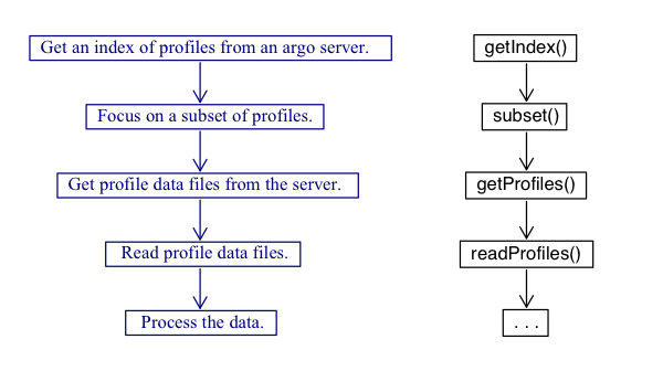
Figure 1 illustrates the typical workflow with the package, with descriptions of the steps on the left, and names of the relevant functions on the right.

Figure 1: Work flow of the argoFloats package with descriptions on the left and relevant functions on the right

As shown above, the central functions for the argoFloats package are getIndex(), subset(), getProfiles(), and readProfiles().

Some built-in data sets are provided for concreteness of illustration and for testing, but actual work always starts with a call to getIndex() to download a full index of float data, which we will demonstrate later in this vignette.

To begin to get familiar with how the argoFloats package works, we will begin looking at the built in data sets. Built into the argoFloats package is the index, indexBgc, indexSynthetic, and indexDeep indices, referring to core Argo, BGC-Argo, a combination, and deep Argo respectively. It should be noted that as of September 21, 2020, indexMerged no longer exists as the switch to indexSynthetic has been made. For the sake of this vignette we will focus on the index data set.

The first step is to access the required packages that will be needed during this tutorial, with

library(oce)
library(ocedata)
library(argoFloats)

To access the embedded index within argoFloats, the following code is used:

data("index")

It is now possible to process the downloaded index using the argoFloats specialized versions of R “generic” functions, plot(), [[, summary(), and show() as shown below.

Processing Steps

The following subsections use built-in data.

Plotting

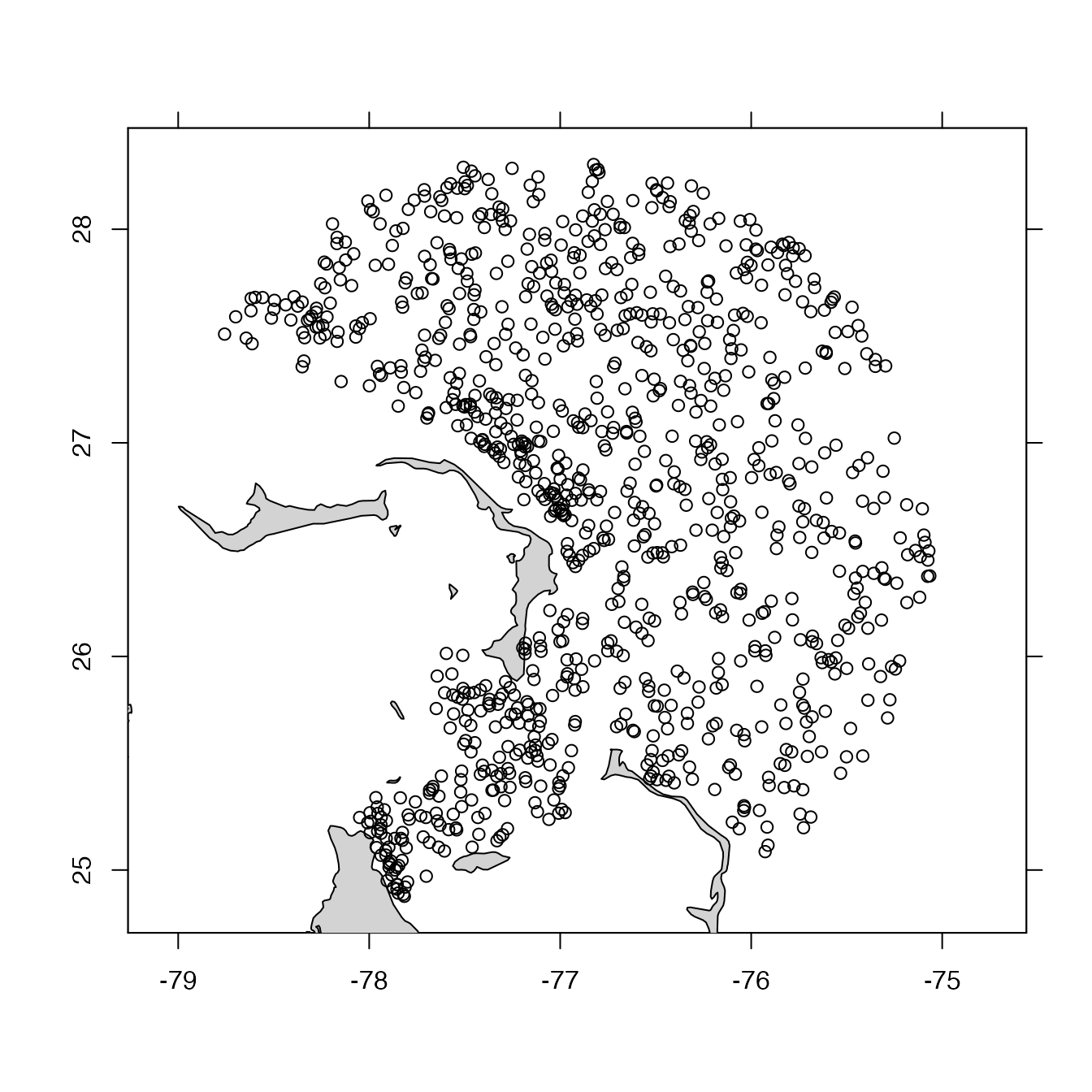
The specialized plot() command within the argoFloats package provides simple ways to plot aspects of argoFloats-class objects. To produce the built in plot and visualize the coordinates of a section of Argo floats off of the Bahamas, the following code is used:

plot(index, bathymetry=FALSE)          # also, try using bathymetry=TRUE

Figure 2: Built in index demonstrating Argo profiling floats within 200 km of Bahamas.

Extracting Data

Furthermore, the [[ command provides a way to extract items from argoFloats objects, without getting lost in the details of storage. For example, if the user wanted to extract the file within the index data set, instead of doing index@data$index$file, instead they can simply do index[["file"]]. (Note that [[<- is not specialized, since the user is highly discouraged from altering values within argoFloats objects).

Summarizing

Additionally, the summary() command displays key features of argoFloats-class objects such as the type, server, file, URL etc. See summary,argoFloats-method() further details.

Printing

Lastly, the show() command provides a one-line sketch of argoFloats-class objects. This gets used by the print() function. For example if the user types in:

index

The following output occurs:

argoFloats object of type "index" with 953 items

Hint: This command can be particularly useful when doing the merge() command, which will be explained in greater detail further down.

It should be noted that the profile elements within argoFloats objects are stored as in the form of argo objects as defined by the oce package. This means that argoFloats users can rely on a wide variety of oce functions to analyze their data. The full suite of R tools is also available, and the vastness of that suite explains why argoFloats is written in R.

Function Details

getIndex()

Until this point, we have demonstrated how the user can become familiar with embedded indices. As previously described, however, actual work always starts with downloading a full index of float data. As shown by Figure 1, the getIndex() command is used to get an index of available Argo float profiles, either by downloading information from a data repository or by reusing an index (stored as an .rda file) that was prepared by a recent call to the function.

The getIndex() command works by specifying the server, with first trying the Ifremer server and then the USGODAE server if that does not work. The next step is to specify the file name. The table below can be obtained using ?getIndex(). As shown, the user has the ability to write the specific file name from the server, or to simply use the embedded nicknames within the package: "core", "bgc" or "bgcargo", or "synthetic". The following table summarizes the contents of the various files indicated by the filename argument.

File Name	Nickname	Contents
`ar_greylist.txt`	-	Suspicious/malfunctioning floats
`ar_index_global_meta.txt.gz`	-	Metadata files
`ar_index_global_prof.txt.gz`	`"core"`	Argo data
`ar_index_global_tech.txt.gz`	-	Technical files
`ar_index_global_traj.txt.gz`	-	Trajectory files
`argo_bio-profile_index.txt.gz`	`"bgc"` or `"bgcargo"`	Biogeochemical data (without S or T)
`argo_bio-traj_index.txt.gz`	-	Biogeochemical trajectory files
`argo_synthetic-profile_index.txt.gz`	`"synthetic"`	Synthetic data, successor to `"merge"`

Additionally, the destdir argument has a default of ~/data/argo, where it should be noted that ~ is a short cut for C:\Users\. See ?getIndex() for further description about the additional arguments for this command.

To get the index from the Ifremer server, the following code is used:

ai <- getIndex("core")

subset()

As shown by Figure 1, the next step when working with the argoFloats package is to use the subset() function to focus on a subset of profiles. The argoFloats package provides tools to sift through profiles based on ID, time, geography, variable, institution, ocean, dataMode, cycle, direction, profile, dataStateIndicator, section, etc.

For geographic subsetting, the user has the ability to subset by circle, rectangle, polygon, or section.

To subset for specific groups of Argo profiling floats off the coast of Bahamas, the following code is used:

# Subsetting by circle
aiCircle <- subset(ai, circle=list(longitude=-77.5, latitude=27.5, radius=50))
# Subsetting by polygon
lonPoly <- c(-76.5, -76.0, -75.5)
latPoly <- c(25.5, 26.5, 25.5)
aiPoly <- subset(ai, polygon=list(longitude=lonPoly, latitude=latPoly))
# Plotting the subsets together
CP <- merge(aiCircle, aiPoly)
plot(CP, bathymetry=FALSE)             # also, try using bathymetry=TRUE

Figure 3: 50 km radius and polygon subset of Argo profiling floats found off the coast of Bahamas

Exercise 1: Use the subset by rectangle function to add a rectangle subset onto Figure 3 and subset all of the data to only include samples between 2012 and 2020.

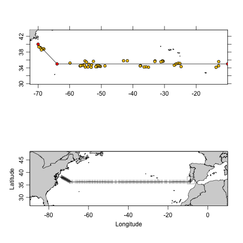
As of March, 2021, a subset by section was developed to create a section of Argo data, similarly to what is done with CTD data. A subset by section combined with subset by time can provide insightful information of Argo vs CTD sampling efforts. An example of this is highlighted below, which compares a section of Argo data from the Mediterranean outflow region across to North America to the line A03 CTD section data collected in 1993-09-11.

Exercise 2: Use the information from Figure 4 to compare Argo and CTD section sampling methods.

library(oce)
library(argoFloats)
oldpar <- par(no.readonly=TRUE)
par(mfrow=c(2,1))
data(section, package="oce")
#getIndex()
ai <- getIndex()
#subset by section
lonlim <- c(-70, -64,-10)
latlim <-c(40,35,35)
index1 <- subset(ai, section=list(longitude=lonlim, latitude=latlim, width=100))
#subset by time
from <- as.POSIXct("2020-09-23", tz="UTC")
to <- as.POSIXct("2020-10-25", tz="UTC")
index2 <- subset(index1, time=list(from=from, to=to))
plot(index2, bathymetry=FALSE,  asp=1/cos(mean(range(unlist(index2[["latitude"]]), na.rm=TRUE))*pi/180),  mgp=getOption("oceMgp")
)
points(lonlim, latlim, pch=21, col="black", bg="red", type="o")
plot(section, which="map", col="tan")
par(oldpar)

Figure 4: Comparison of Argo vs. CTD section data in a westward transect from the Mediterranean outflow region across to North Atlantic. Top: Argo data including 49 samples from 2020-09-23 to 2020-10-25 made by the argoFloats package. Bottom: Line A03 section including 124 CTD samples from 1993-09-23 to 1993-10-25 made by oce package

getProfiles()

The next step within the argoFloats package is the getProfiles() function. This takes an index constructed with getIndex(), possibly after focusing with subset,argoFloats-method(), and creates a list of files to download from the server named in the index. Then these files are downloaded to the destdir directory, using filenames inferred from the source filenames. The value returned by getProfiles() is suitable for use by readProfiles() function.

readProfiles()

The readProfiles() command works with either a list of local NetCDF files, or a argoFloats object type profiles, as created by getProfiles().

The command can be useful for analyzing individual profiles, for example:

index1 <- subset(index, 1:2) # To subset for profiles
profiles <- getProfiles(index1)
argos <- readProfiles(profiles)
argosClean <- applyQC(argos)
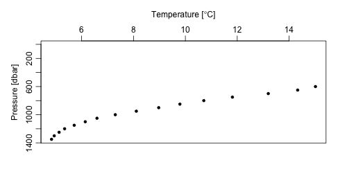
plot(argosClean, which="profile", type="p")

Figure 5: Temperature profile created using argoFloats readProfiles function

Exercise 3: Using the profile in the previous example, plot a TS diagram.

Appendix 1: Work Flow With Local Index Files

In normal usage, getIndex() works by downloading a gzipped CSV file (with suffix .gz) from an Argo server, analyzing that file writing an R Data Archive file (with suffix .rda), and then deleting the .gz file. However, if getIndex() is called with the parameter keep set to TRUE, it will retain the .gz file in the directory named by the destdir argument. This can be useful if there is a need to work with the data in a processing system other than argoFloats.

It is possible to instruct getIndex() to skip remote downloads, to instead use a local .gz or .rda file. This is done by providing the file name as the first argument, and by setting server=NULL, e.g. using

index <- getIndex("~/data/argo/ar_index_global_prof.txt.gz", server=NULL)

index <- getIndex("~/data/argo/ar_index_global_prof.rda", server=NULL)

after which the other processing steps, as outlined in the previous section, can be followed.

The .rda approach is better than the .gz one, for two reasons: (1) it is faster and (2) it usually sets a better foundation for later calls to getProfiles(). The second factor is a result of the fact that the .gz files on servers do not contain an indication of the server URL, whereas the locally-generated .rda files do so. (Recall that getIndex() can try a list of servers, and it records in the .rda file the first one that yielded results from a download attempt.)

Whether the .gz or .rda method is chosen, it is worth noting that index files go out of date, as new data become available, and also as pointers to real-time data are made obsolete because of replacement by delayed-mode equivalents. Even so, it can be a good idea to download an index file before a classroom/workshop exercise and to share it over a local network, avoiding placing too much stress on the larger network.

Solutions to Exercises

Exercise 1: Use the subset by rectangle function to add a rectangle subset onto Figure 3 and subset all of the data to only include data between 2012 and 2020.

library(argoFloats)
ai <- getIndex()
# Subset by circle
index1 <- subset(ai, circle=list(longitude=-77.5, latitude=27.5, radius=50))
# Subset by polygon
lonPoly <- c(-76.5, -76.0, -75.5)
latPoly <- c(25.5, 26.5, 25.5)
index2 <- subset(ai, polygon=list(longitude=lonPoly, latitude=latPoly))
# Subset by rectangle
lonRect <- c(-76.5, -76)
latRect <- c(27, 28)
index3 <- subset(ai, rectangle=list(longitude=lonRect, latitude=latRect))
# Merge the subsets together
index4 <- merge(index1, index2)
index5 <- merge(index3, index4) # Note right now can only merge 2 indices together
# Subset for year 2012-2020
index6 <- subset(index5, time=list(from="2012-01-01", to="2020-01-01"))
# Plot data
plot(index6, bathymetry=FALSE)             # also, try using bathymetry=TRUE

Exercise 2: Use the information from Figure 4 to compare Argo and CTD section sampling efforts.

Figure 4 reveals that it takes almost 3 months of Argo sampling to reproduce a 1 month CTD section cruise. Additionally, it displayed that there are geographical gaps within the Argo data. On the other hand, it should be noted that by extending the latitude range, these gaps are quickly filled in. In conclusion, Argo sampling is much more cost effective, and it can allow for collection of more information (i.e. nutrients, oxygen, backscattering, etc.) if such thing is desired.